Data Lineage in DAX

Data lineage is a feature of DAX that most developers don’t know exists when they use it. This article focuses on data lineage in DAX and how it can help us generate better DAX code. Before diving into our article, let’s figure out what is data lineage.

What’s data lineage?

First, data lineage is a tag assigned to each column in a table that identifies the original column in the data model that produced the column value. For example, the following query returns the different categories in the product table:

The result contains 8 lines, one for each category:

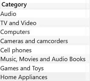
Return a table containing 8 strings via the VALUES function. However, they are not just strings. DAX knows that these strings originate from the Product[Category] column. So, as columns of the Product table, they inherit the ability to filter other tables in the model after the filter is propagated through the relationship. That’s why the context switch iterates VALUES ( Product[Category] ) to filter the Sales table. Let’s look at the following query:

The query result contains the sales value for each product category:

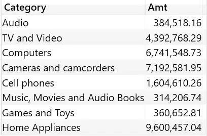
The string “Audio” by itself cannot filter the Sales table. You can easily check this result by running the following query:

EVALUATE VAR Categories = DATATABLE ( “Category”, STRING, { { “Category” }, { “Audio” }, { “TV and Video” }, { “Computers” },
{ “Cameras and camcorders” }, { “Cell phones” }, { “Music, Movies and Audio Books” }, { “Games and Toys” }, { “Home Appliances” } } )
RETURN ADDCOLUMNS ( Categories, “Amt”, [Sales Amount] )

The latter query returns the same value for all rows in the Amt column:

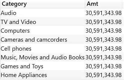
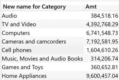
Neither column names nor column contents matter. All that really matters is the data lineage of the column, which is the original column from which the value was retrieved. (That is, data lineage refers to the fact that regardless of the column name and column content, its retrieved value is the original column.) If a column is renamed, data lineage is still maintained. In fact, the query below returns a different value for each row:

EVALUATE ADDCOLUMNS ( SELECTCOLUMNS ( VALUES ( ‘Product'[Category] ), “New name for Category”, ‘Product'[Category] ), “Amt”, [Sales Amount] )

The “New name for Category” column still maintains the data lineage of Product[Category]. Therefore, even though the column names in the results are different from the original column names, the results still show sales by category.

Data lineage is maintained as long as the expression is generated by column references only. For example, adding an empty string to Product[Category] in the preceding expression would not change the column contents, but would break data lineage. In the code below, the source of Category’s new name is an expression, not just a column reference. Therefore, the new column has new data lineage independent of any source columns of the model.

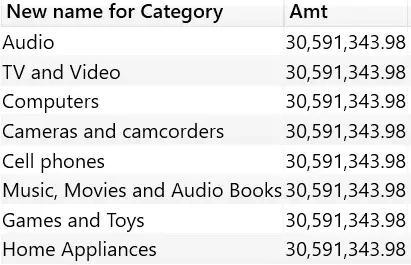
EVALUATE ADDCOLUMNS ( SELECTCOLUMNS ( VALUES ( ‘Product'[Category] ), “New name for Category”, ‘Product'[Category] & “” ), “Amt”, [Sales Amount] )

The result is as expected, the Amt value is the same for all rows:

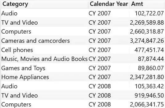
Each column has its own data lineage, even if a table contains columns from different tables. Therefore, the results of a table calculation can apply filters to multiple tables at the same time. It can be clearly seen in the query below which contains Product[Category] and Date[Calendar Year]. Both columns apply their filtering to the Sales Amount measure through the filtering context resulting from the context transformation.

The results show the Sales amount values ​​of different categories and years. Both Product[Category] and Date[Calendar Year] filter the Sales Amount metric.

Even though data lineage is performed by the engine in a fully automated fashion, developers can choose to change the data lineage of a table. TREATAS can do this work. TREATAS accepts the table as its first parameter, and the second parameter is the column in the table (TREATAS, which means TREAT AS, can be understood as [treat parameter 1 as parameter 2]).

TREATAS returns the same input table, each column marked with the data lineage referenced by the column specified as parameter. If some values ​​in the table contain values ​​that do not correspond to valid values ​​in the columns used to apply data lineage changes, TREATAS will cull those values ​​from the input.

For example, the query below builds a table with a list of strings, one of which is “Computers and geeky stuff” that is not associated with any of the categories in the model. We use TREATAS to force the data lineage of the table to Product[Category].

EVALUATE VAR Categories = DATATABLE ( “Category”, STRING, { { “Category” }, { “Audio” }, { “TV and Video” },
{ “Computers and geeky stuff” }, { “Cameras and camcorders” }, { “Cell phones” }, { “Music, Movies and Audio Books” },
{ “Games and Toys” }, { “Home Appliances” } } )
RETURN ADDCOLUMNS ( TREATAS ( Categories, ‘Product'[Category] ), “Amt”, [Sales Amount] )

The result contains Sales Amount by category, but the line with Computers and geeky stuff is missing from the output.

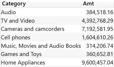
When there is no category named “Computers and geeky stuff” in the data model, so TREATAS must cull that row from the output to complete the data lineage transformation.

Perform Data Lineage

Now we understand what data lineage is and how to perform data lineage using TREATAS. Now let’s look at an example where the DAX code generated by TREATAS and data lineage requires that the Sales Amount be calculated only on the first day of sale for each product. The same calculation would make sense for customer, store, or any other dimension, but for now only consider products in this example.

Since each product has a different first sale date, the first approach is to calculate the first sale date iterating on a per-product basis, then calculate the Sales Amount for that date, and finally aggregate the results for all products, with the following code:

FirstDaySales v1 := SUMX ( ‘Product’, VAR FirstSale = CALCULATE ( MIN ( Sales[Order Date] ) )
RETURN CALCULATE ( [Sales Amount], ‘Date'[Date] = FirstSale ) )

Here is the code return result:

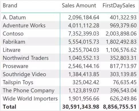
The result is correct, but the code above is not optimal because it iterates over the Product table, generating context transitions for each product, and applying filters on dates, without exploiting any relationships, with relatively low performance. Below we will see that other computations of this metric attempt to achieve the same result in a more performant manner.

The first step in the calculation of the second way is to build a table containing the product name and the corresponding date of the first sale, then use this table to apply a filter to Sales, the code below is an improvement compared to the previous piece of code, but still Not optimal because SUMX still generates a context transition per product:

FirstDaySales v2 :=
VAR ProductsWithSales =
SUMMARIZE ( Sales, ‘Product'[Product Name] )
VAR ProductsAndFirstDate =
ADDCOLUMNS ( ProductsWithSales, “Date First Sale”, CALCULATE ( MIN ( Sales[Order Date] ) ) )
VAR Result = SUMX ( ProductsAndFirstDate, VAR DateFirstSale = [Date First Sale]
RETURN CALCULATE ( [Sales Amount], ‘Date'[Date] = DateFirstSale ) )
RETURN Result

But if the variable ProductsAndFirstDate generated by the ADDCOLUMNS function can be used as the filter parameter of CALCULATE, which will filter a product table and a date table, this version will perform better (unfortunately, it is wrong):

FirstDaySales v3 (wrong) :=
VAR ProductsWithSales = SUMMARIZE ( Sales, ‘Product'[Product Name] )
VAR ProductsAndFirstDate = ADDCOLUMNS ( ProductsWithSales, “Date First Sale”, CALCULATE ( MIN ( Sales[Order Date] ) ) )
VAR Result = CALCULATE ( [Sales Amount], ProductsAndFirstDate )
RETURN Result

The above code does not have the iterative operation of SUMX, but this version of the code is buggy because it returns the same Sales Amount value without applying any filters.

In fact, the variable ProductsAndFirstDate generated by ADDCOLUMNS contains a product and a date, but in terms of data lineage, the product name inherits the data lineage of Product[Product Name], but the Date First Sale column inherits Sales[Order Date] The data lineage, instead, produces the result of the MIN expression. The Date First Sale column has its own data lineage, independent of other tables in the data model.

The correct optimization metric is as follows:

FirstDaySales v4 :=
VAR ProductsWithSales = SUMMARIZE ( Sales, ‘Product'[Product Name] )
VAR ProductsAndFirstDate = ADDCOLUMNS ( ProductsWithSales, “First Sale”, CALCULATE ( MIN ( Sales[Order Date] ) ) )
VAR ProductsAndFirstDateWithCorrectLineage = TREATAS ( ProductsAndFirstDate, ‘Product'[Product Name], ‘Date'[Date] )
VAR Result = CALCULATE ( [Sales Amount], ProductsAndFirstDateWithCorrectLineage )
RETURN Result

The above solution is not the primary solution for the model. However, in terms of performance, this code is nearly optimal, perhaps because we didn’t find a better performing version — if you do, we’d like to see it in the comments. Once you are familiar with data lineage, you can think like the solution above and understand how filters use data lineage to pass from one table to another.

Conclusion

Understanding data lineage is crucial for DAX developers, and while it’s not as directly related as row context, filter context, and context transformation, it’s certainly a skill that must be understood to be a professional DAX developer.

Thank you for reading our article and hope it can let you have a better understanding of data lineage in DAX. If you want to learn more about data lineage, we would like to advise you to visit Gudu SQLFlow for more informations. As one of the best data lineage tools available on the market today, Gudu SQLFlow can not only analyze SQL script files, obtain data lineage, and perform visual display, but also allow users to provide data lineage in CSV format and perform visual display.